

LasVegas
2D Monte Carlo Tool
Welcome to the 2D Monte Carlo code for device simulation LasVegas !
In the following you will learn how to use the tool and how to run the simulations for your device structure. For now on, Client is the computer where you are running the browser (your local computer) while Server is the computer where you are connected (ICODE server).
The detailed manual for the LasVegas input file can be found in: LasVegas Manual
There are 5 simple steps to follow for a complete device simulations. These are:- Login
- Select working directory
- Run the MonteCarlo simulation tool
- Run the device definition and simulation wizard
- Monitoring the job execution
- Plot the result
Step 1 & Step 2: Login and Select working directory
For the first two steps see the detailed instructions in the documentation file: Accessing ICODE system.Step 3: Run the Monte Carlo Simulation Tool
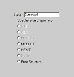
By having selected a well defined working directory you can now run the Monte Carlo simulation tool. Click on the LasVegas icon and a window like that in left down figure will appear.
|
Select
on of the possible structure of the device you would simulate. As you
can see not all the option are possible. These functionalities will be
implemented in future release of the tool.
LasVegas (the name of this Monte Carlo simulator) is an interactive simulation tool developed at TU-Munich and in Roma Tor Vergata, to simulate electronic devices, FET transistors (actually HEMT and MESFET), BJT transistors (not jet implemented), diodes etc. It uses a Monte Carlo algorithm, and allows to choose among a wide range of conditions. The GUI (Graphical User Interface) is realized in Java and we tried to make it easy to use. It is still under development, and suggestions will be welcome for its improvement. |
There are two ways to run LasVegas:
- You edit directly the input file. In this case chose the button Free Structure and then edit the input file changing the template. In order to properly change the input file you may need to read the LasVegas Manual. This way is much more complicated with respect to the following one however it allows you to use LasVegas for very complicated situations.
- You can use the GUI as discussed in the following Step 4.
Step 4: Run the Device Definition and Simulation wizard
|
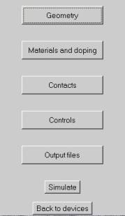
If you would avoid to enter the device structure directly in the Monte Carlo input file you can use the GUI wizard. Click on the device structure you would simulate. For the case of the HEMT structure a window like this will show up The six buttons (Geometry, Materials and Doping, Contacts, Controls, Output files, Simulate) when pressed will open new windows where you can define the device structure and the simulation. Generally, you should call these definitions consequently starting from the Geometry definition. |
|
Geometry:
|
|
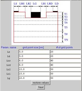
The Geometry frame is shown in the right figure. Here you define the horizontal structure (contacts and air regions) and the vertical structure (layers) of your device. In a first card you set the horizontal regions (contacts, source, gate, drain and air regions). You have to define, for each region the number of grid points (# of grid points) and the size of each grid point (grid point size). The total length of the region = grid point size X # of grid points. If you push the next button you will access the next table. |
|
|
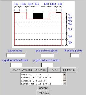
This frame is shown in the left figure. For each layer you have to provide a name, the number of vertical grid points (# of grid points), the size in nm of each vertical grid point (grid point size). The total thickness of the layer = grid point size X # of grid points. For both horizontal and vertical grids you can define the reduction ratio (the number of grid points divided by the reduction ratio gives the number of cells effectively used in the simulation, see LV manual). You can exchange the position of the layers (click on the swap layers button, the click on the first layer, the click on the second layer to swap and so on. To end, click once more on the swap layers button), update an existing layer (click on the layer in the list, then change the parameters and click update), delete a layer. |
|
|
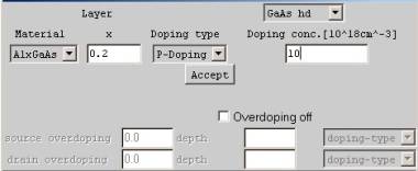
Materials:
|
|
For
each layer (you can select it from the bottom list in the frame), you
choose the material type (left list), concentration, doping type,
doping concentration, as well as device-dependent characteristics like
Overdoping (to better simulate contacts) under contacts for HEMT or
ionic implantation profiles for MESFET. To define Overdoping choose the type of doping, the doping value (in units 1018 cm-3) and the vertical (y) grid point down to where the Overdoping extends. |
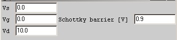
Contacts:
|
here you define the applied voltages at contacts and the barrier high for the Gate Schottky contact.
|
|
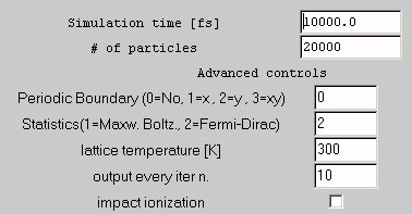
Controls:
|
here you define all the physical parameters for the simulation, like boundary conditions, temperature, activation of impact ionization etc. |
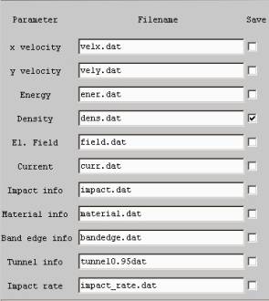
Output:
here you choose which data produced by the simulation you want to save on the disk. Some of the files will be further splitted in subfiles for a direct plot with HyperPlot. For example, the density file (in this case '' dens.dat '') contains density for electron in Gamma valley, in L valley in X etc. etc. (see Manual) and this multidata type of file is not handled by HyperPlot (but you can download and use your own data plot tool). Thus the tool automatically split the '' dens.dat '' file in subfiles like '' dens_e_gamma.dat '' for electron in gamma valley. HyperPlot can plot this subfile. |
|
|
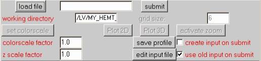
This frame serves to submit the request for the simulation, or to save the input file without starting the simulation, if you want to edit and modify it. |
||
|
You can at this point save the profile of the project (save profile).In this way you create the file LVprofile.ser in your directory. This file contains all your setting of the device (all the project) and can be run directly by pressing with the mouse the start button. In this way you can easily modify your project later on. When LV start the simulation, it reads the file device.ini. When submit the job (submit button) you can create this input file according to your device definition if the create input on submit is marked. Otherwise you can use another (for example manually modified) device.ini input file present in the working directory if use old input on submit is marked |
Step 5: Monitoring the job execution
After the job has been submitted you can monitor the job execution by clicking on the Jobs Status link in the left frame, just above the list of the Services (simulators). For details on this see the relative documentation: Job Monitor Utility.Step 6: Plot
Results of the simulation can be either downloaded on the CLIENT computer or plotted using the ICODE Hyperplotter tool. For reference see the relative documentaton file: Hyperplotter Graphic Utility.