Green-Density Functional Tight-Binding (gDFTB): short manual

Aldo Di Carlo and Alessandro Pecchia

INFM-Dipartimento di Ingegneria Elettronica, Università di Roma ``Tor Vergata'', 00133 Roma, Italy

RULES TO GENERATE THE MOLECULAR STRUCTURE

DEFINITION OF THE PROBLEM

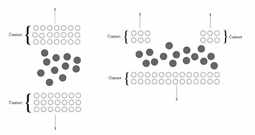
Let us define the system we would like to describe. This system can be generally divided in two parts:

1. the contacts
2. the molecular region.

The contacts represent semi-infinite leads that end on the molecular region (see Fig. 1.). On the other end, the molecular region can be any kind of atom collection that represents the system we would like to study (for example the active part of a device or the molecule we would like to study via STM).

Figure 1: Typical molecular structure where current can flow.

Contacts and molecular region should be treated in different ways so we need to clearly identify such separation in our system. We will be interested to the molecular system, but the effects of the contact will enter in such description via self-energy terms as we will describe in the following.

CONTACTS

Strictly speaking we would like to describe the molecular system by using special (open) boundary condition for the Kohn-Sham equation. Usually, we will describe a molecule just defining the atoms that form the molecule itself. For the description of a crystal one use the Bloch theorem to reduce the calculation to few atoms. However, to describe the current we need to define semi-infinite contacts that inject/receive current through/from the molecular region. In other words we need to define open boundary condition to our problem. Usually, this can be obtained in the context of scattering theory as it has been done by the group of Ratner, via the transfer matrix or, as we do, via the Green's function technique.

In order to define the contacts it necessary to define the Principal Layer (PL). The principal layer is defined as in the following:

1. It is represented by a sequence of atoms or atomic planes (depending on the dimensionality of the contact). The interaction between principal layers is nearest-neighbors, that is, each PL interact only with the adjacent PL.
2. It represents a unit cell of the semi-infinite crystal forming the contact.In gDFTB the typical interaction radius is about 4Å. Thus, a PL should be large at least 4 Å in order to ensure that the interactions between PL are nearest-neighbor (condition II). Such definition of PL is sufficient for an easy calculation of the surface Green function needed in the program.

WHICH ARE THE INPUT FILES NEEDED TO RUN gDFTB ON ICODE ?

To run gDFTB on ICODE server you need only to define the input atomic structure in a PDB file (you may also describe the system via XYZ but then you have to convert to PDB by using the built-in filter on ICODE)

An accurate ordering of the atoms inside the PDB file is strictly necessary. In the following we will outline the rule for atom ordering.

HOW TO DEFINE THE ATOMIC POSITION FILE

In order to create the atomic position file it is better to work in the XYZ format and the use the ICODE filter to generate the PDB file. The typical XYZ file has the following format

Numer_of_atoms

(blank line)

Atom_type X Y Z

Atom_type X Y Z

.

.

.

Let's call structure.xyz the atomic position file.

To let gDFTB running in a correct way we need to order the atoms in structure.xyz in the following order (from first to last):

• Atoms belonging to the molecular region.
• Atoms belonging to the first contact. Each contact should be represented by two PL. Thus, first you have to write the atoms belonging to the first PL (the one closer to the molecule) than the atoms belonging to the second PL. Since PLs are unit cell of the system, you should order the atoms in the two PLs consistently (that is, you should number the atoms in the second PL like the atoms in the first PL plus the offset, or in other words, the sequence of atoms in the second PL should match the sequence of atoms of the first PL).
• Atoms belonging to the second contact (with the same rules for PLs as described above and reminding that the first PL of this second contact is that closer to the molecular region)

One should take care that contacts do not see each other, that is the distance between contacts should be larger that 4 Å. A typical system is shown in figure 2.

Figure 2. Typical system where current calculation is performed.

The atoms in the middle belong to the molecular region while the other atoms belong to contacts. Here, each ring of the contact plus the left and right C atom forms a PL.

Here is the corresponding structure.xyz file:

---------------------

60

C -3.295718 0.05738 0.02231

C -1.85143 0.057275 0.02231

H -1.694709 -2.115839 0.02231

H -1.693445 2.230373 0.02231

C -1.144662 -1.165542 0.02231

C -1.144014 1.279731 0.02231

C 0.24859 -1.165769 0.02231

C 0.249297 1.279115 0.02231

H 0.798012 -2.116683 0.02231

H 0.799313 2.229678 0.02231

C 0.955785 0.056462 0.02231

C 2.400341 0.056149 0.02231

C 3.62002 0.057381 0.02231

C 5.064598 0.05741 0.02231

H 5.221552 -2.115661 0.02231

H 5.222018 2.230359 0.02231

C 5.771574 -1.165499 0.02231

C 5.77192 1.280113 0.02231

C 7.164536 -1.1656 0.02231

C 7.164891 1.279826 0.02231

H 7.713435 -2.116654 0.02231

H 7.713947 2.230795 0.02231

C 7.871766 0.056998 0.02231

C 9.316176 0.056828 0.02231

C 10.535499 0.057162 0.02231

C 11.979927 0.056796 0.02231

H 12.136415 -2.117302 0.02231

H 12.137854 2.230735 0.02231

C 12.686001 -1.166297 0.02231

C 12.686849 1.279386 0.02231

C 14.078736 -1.167429 0.02231

C 14.079566 1.279485 0.02231

H 14.629369 -2.117156 0.02231

H 14.63085 2.22883 0.02231

C 14.783592 0.055782 0.02231

C 15.87355 0.055763 0.02231

C -4.515436 0.055976 0.02231

C -5.96006 0.056341 0.02231

H -6.116344 2.229305 0.02231

H -6.118073 -2.11668 0.02231

C -6.66685 1.279377 0.02231

C -6.667658 -1.166223 0.02231

C -8.05966 1.279803 0.02231

C -8.060467 -1.165627 0.02231

H -8.608259 2.231079 0.02231

H -8.609987 -2.116372 0.02231

C -8.767195 0.057318 0.02231

C -10.211617 0.057582 0.02231

C -11.430935 0.056007 0.02231

C -12.875274 0.056261 0.02231

H -13.031527 2.230274 0.02231

H -13.033652 -2.117722 0.02231

C -13.581262 1.279515 0.02231

C -13.582379 -1.166339 0.02231

C -14.97409 1.28071 0.02231

C -14.9752 -1.166165 0.02231

H -15.52444 2.230593 0.02231

H -15.526652 -2.115432 0.02231

C -15.678999 0.057615 0.02231

C -16.7689 0.058013 0.02231

---------------------

As you see, the first 12 atoms belong to the molecular region. After these there are the 24 atoms (12 for each PL) of the right contact and then other 24 atoms of the left contact. Another system is shown in Fig.3 where an explicit indication of PL and molecular region is shown.

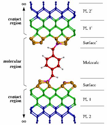
Figure 3. Layer definition example - A benzene molecule with a CH ligand is placed between two reconstructed diamond contacts.

OUTPUT FILES

The output files are those of DFTB plus the following files:

Conductance calculations:

• conductance.dat. The molecule conductance: Col1=energy[eV]; Col2=transmission coefficient.
• surfdens_01.dat. The surface density of states of the first contact: Col1=energy[eV]; Col2=surface density of the states [arb. units].
• surfdens_02.dat. The surface density of states of the second contact: Col1=energy[eV]; Col2=surface density of the states [arb. units].

Current Calculations

• IV.dat. The current voltage characteristics: Col1=Potential[V]; Col2=Current [A].

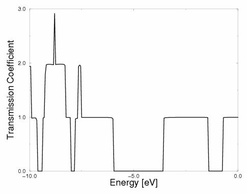
Figure 4. Calculated conductance (= transmission coefficient) for the structure of Fig.2. Channels of conductance are clearly visible.

RUNNING THE CALCULATIONS

Submit the job via the gDFTB CONTROL interface.