

QCL2000
Schrödinger-Poisson and Monte Carlo simulation of Quantum Cascade Lasers
QCL2000 is a Ensamble Monte Carlo simulation tool, based of a non-parabolic effective mass Schrödinger Poisson solver for the calculation of the electron energies and wavefunctions.
From now on, Client is the computer where you are running the browser (your local computer) while Server is the computer where you are connected (ICODE server).
There are 5 simple steps to follow for a complete device simulation. These are:
- Login
- Select working directory
- DEFINE THE SIMULATION PARAMETERS
- RUN The simulation
- Monitoring the job execution
- Plot the result
Step 1 & Step 2: Login and Select working directory
For the first two steps see the detailed instructions in the documentation file: Accessing ICODE system.Step 3: DEFINE THE SIMULATION PARAMETERS
After login and selection of your working directory, you are ready to choose the simulation tool: click on QCL2000 in the Device Simulators frame and the simulation interface opens in a new window.
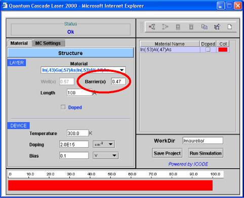
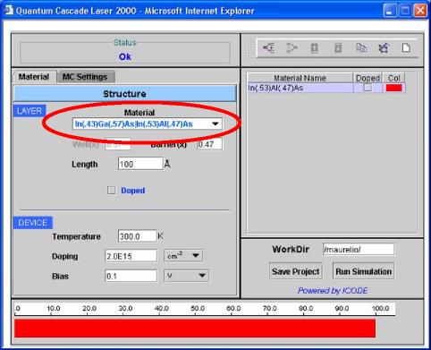
| 1) Select the name for the device materials from the Material menu, as shown in the window. |
|
| Fig.1 | |
|
2) Select the alloy concentration of the material in Well and Barrier, respectively Well(x) and Barrier(x). For instance, as shown in Figure 2, a couple of materials In0.43Ga0.57As/In0.53Al0.47As has been selected for Well/Barrier. The alloy concentration of Ga in Well is Weel(x)=0.57, Alloy concetrantion of Al in Barrier is Barrier(x)=0.47.
|
 |
|
Fig. 2
|
|
|
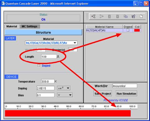
3) Let's begin to define the Leghts of the layers in the growth direction of the device. As default, the structure must begin with a barrier, which is identified in the right frame with a red colour, the well being identified by a bue colour. The thickness of each layer in Angstrom must be provided in the appropriate field Lenght (red elipse in Figure 3). The arrows show the layer visualization in the wizard: in the right frame, the device constructor, and in the bottom frame, the unidimensional graphical rappresentation of the device.
|
 |
|
Fig. 3
|
|
|
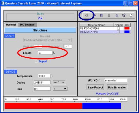
4) Let's proceed to insert sequentially the following layers, by means of the blu circled botton: the add botton (see Figure 4). For each layer the Lenght must be defined in the red circled field. Consider that in the device, well and barrier layers will be added alternatively in a automatic way when you push the add button, and that the device must end with a barrier. If these requirements are not satisfied the simulation cannot start.
|
 |
|
Fig 4
|
|
|
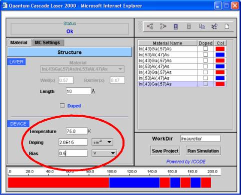
5) When the structure has been completed, the simulation parameters must be defined: Temperature (in K), Doping (2D doping in cm-2 or 3D doping in cm-3), and the Applied Bias (in V) or the Electric Field (in KV/cm).
|
 |
|
Fig. 5
|
|
|
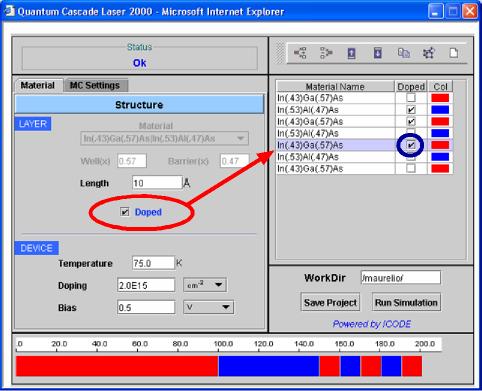
6) One must now proceed to define the doped layers. As can be seen in Figure 6, you can select a material from the right frame device constructor list, and simply click on the appropriate checkbox Doped, in the left frame of the wizard (red circled). Automatically, in the Material Name list, the respective layer will be shown as "doped" (blue circled Doped box). This layer will be considered doped.
|
 |
|
Fig. 6
|
|
|
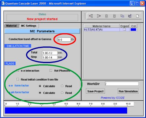
7) In the MC Settings section, the Monte Carlo Parameters for the simulation must be setted, as you can see in Figure 7: the Conduction Band Offset in eV, COB, must be written in the field inside the red circle The SIMULATION TIME Parameters are:
Suggested values for the parameters are a Timestep on 1.0E-14 s, and a total time less than 1.0E-10 (100 ps). In one need longer simulation time, it is convenient to execute sequentially shorter simulations (of 10/20 picoseconds), taking care to select Read initial condition from file in the FLAGS area. Here one can decide to include the calculation of electron-electron scattering (e-e interaction), and the Hot Phonon population in the phonon statistics. The first time you runa simulation for a structure you need to calculate the e-e and e-ph (electron-Optical Phonon) form factor (it may need hours, depending on your device). If you run successive simulations without changing the device structure and applied bias, then you can choose to read e-e and e-ph form factors from file, already calculated and saved in the previous run, this resulting in a sensible saving of time.
|
 |
|
Fig. 7
|
|
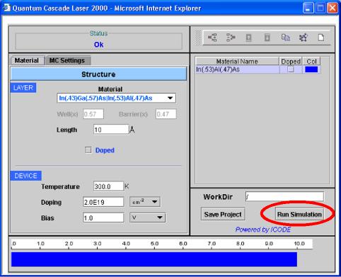
Step 4: run the simulation
|
8) Now the setting is complete. Go to Material section and start the simulation clicking on the Run Simulation button at the bottom-right. The calculation of the electron eigenvalues and eigenfunctions of the structure will be executed. When the simulation stops, the calculated levels will be shown. Thus, a choice of the levels one want to include in the Monte Carlo simulation and the boundary conditions must be done (see points 9-11). Once levels have been selected, the simulation, which now will include the MC, must be started again (see point 12), giving, at the end, the final results. |
|
|
Fig. 8
|
|
|
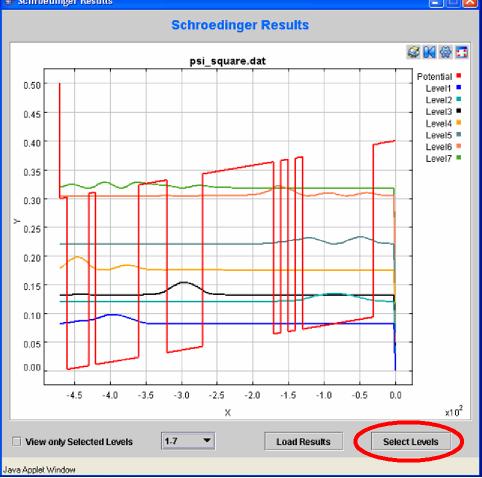
9) When the Schrödinger-Poisson solver reaches the convergence, the provided energy levels and the wavefunctions are automatically plotted in the pop-up window Schrödinger Results. The curves in the plot represent the Potential profile of the Conduction Band of the Gamma Valley, and the square moduli of the wavefunctions, shifted of the relative energy. Levels are numbered from the lowest in energy (Level 1) to the highest calculated. Thus, one can proceed to the choice of the levels to be included in the Monte Carlo Simulation, clicking on the Select Levels button, red circled in Figure 9. |
|
| Fig. 9 | |
|
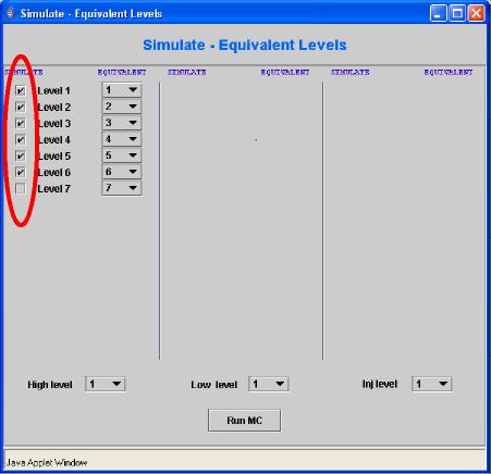
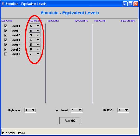
10) Once the button is pressed a new pop-up window Simulate - Equivalent Levels will open, showing the list of the levels calculated in the previous step (Schrödinger-Poisson). Among them one can choose, one by one, the levels wich will be included in the following Monte Carlo Simulation. Usually in the calculations, spurious solution of the Schroedinger Poisson Equation or boundary effects affect the shape of some wavefunctions. This is the reason to exclude such solutions from the MC simulation. To obtain a complete set of wafunction for the MC simulation the device structure must be designed properly, repeating the stage of the QCL (injector + active region) 3/5 times, depending on the total number of layers (the maximum number of layers for this version of QCL2000 is 50). For instance, in Figure 10, the first six levels, of the group of seven previously calculated (and plotted in Figure 9), have been selected, simply clicking in the respective checkbox in the SIMULATE column. Remainder: the levels are numberer on an energy scale, from the lowest (Level 1) to the highest. |
|
| Fig 10 | |
|
11) Thus one can impose the type of boundary condition on the device. This is done defining some Equivalent Levels. If levels i and j are equivalent, the electrons having the level j as final state of a scattering process, will be automatically transferred to the level i, realizing a sort of periodic boundary condition between these two electronic states. If one level is equivalent to itself, than no transferring of electron will be performed. In the example of Figure 11a, only the first two level have equivalent ones: in particular, if an electron transition undegoes to the 1st, it is transfered to the 5th, and from the 2nd to the 6st. This costrain can be used to realize a periodic boundary condition, and the system can be considered as infinite (at least from the point of view of the levels, while the device structure is necessary of finite size), in which the electrons flow continously in the device, until the stationary condition is reached. |
Fig. 11a |
Fig. 11b
|
|
|
12) The last step is to define which are the High Laser level and Low Laser level, among the selected ones. The distribution function will be plotted as output for the level indicated in the field inj level. Now the simulation can start, clicking the button Run MC. |
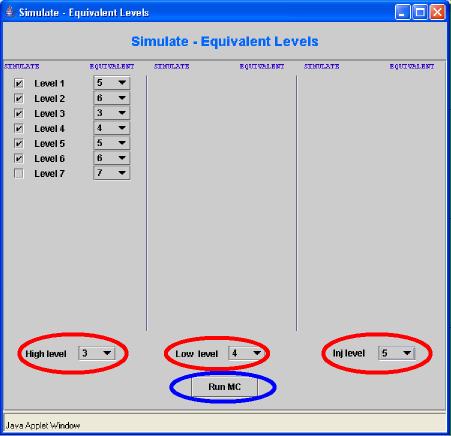
Fig. 12
|
Step 5: Monitoring the job execution
After the job has been submitted you can monitor the job execution by clicking on the Jobs Status link in the left frame, just above the list of the Services (simulators). For details on this see the relative documentation: Job Monitor Utiliy.Step 6: Plot
Results of the simulation can be either downloaded on the CLIENT computer or plotted using the ICODE Hyperplotter tool. For reference see the relative documentaton file: Hyperplotter Graphic Utility.