Green-Density Functional Tight-Binding (DFTB)

Aldo Di Carlo and Alessandro Pecchia

INFM-Dipartimento di Ingegneria Elettronica, Università di Roma ``Tor Vergata'', 00133 Roma, Italy

Welcome to the Documentation File of theDensity-Functional Tight-Binding code DFTB !

The tool allows you to calculate structural, electronic and transport properties of molecules and other nanostructures.

DFTB code has been developed by the Prof. Thomas Frauenheim group at the University of Paderborn (Germany). The DFTB extension for current calculations has been developed by the Optoelectronic group at the University of Rome Tor Vergata .

In the following you will learn how to use the tool and how to run the calculation for your atomic system. For now on, Client is the computer where you are running the browser (your local computer) while Server is the computer where you are connected (ICODE server).

The detailed manual for the DFTB input file can be found in:

• a short DFTB manual;
• the full DFTB manual and developer page

There are 5 simple steps to follow for a complete device simulations. These are:

1. Login
2. Select working directory
3. Rules to generate molecular structure
4. Upload the molecule/nanostructure
5. Plot the atomic system
6. Define simulation parameters
7. Monitoring the job execution
8. Plot the result

Step 1 & Step 2: Login and Select working directory

For the first two steps see the detailed instructions in the help file here.

To generate correctly the molecular structure you are asked to follow few rules. See the detailed instructions in the help file here.

Step 4: Upload the molecule / nanostructure

You have now to upload from the CLIENT to the SERVER the molecule (or nanostructure) description file. For the moment you can use only PDB formatted files. Please use the program BABEL to comvert form other format to PDB format. Use the upload button on the ICODE frame to upload the file.

Step 5: Plot the atomic system

After uploading you can plot the atomic system by pressing the start button right to the PDB file (in our example inrot.pdb). You will obtain something like this.

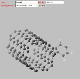
You can rotate the molecule by using mouse action+left click. If you click the controls button a new control window will show up

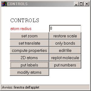
Here you can modify the appearance of the molecule on the molecule viewer. set zoom: zoom in or zoom out the molecule by using mouse action restore scale: restore the scale set translate: translate the molecule on the viewer only bonds: hide the atoms balls compute properties: pop-up a new window for the calculations (see below) edit file: edit the PDB file 3D atoms / 2D atoms: change the rendering of the atoms replot molecule: Replot the molecule put label: show atom names put number: show atom numbers according to the PDB sequence modify atoms: modify the atoms

Step 6: Define computation parameters

To compute molecule properties you need to define some computation parameters. To do this click on the compute properties button of the Controls window. A new window will show-up

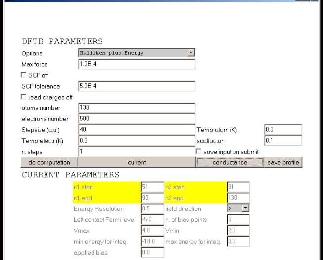
This window is divided in DFTB PARAMETERS and CURRENT PARAMETERS.

While DFTB parameters should always be set, the Current parameter may not be set if current or conductance properties are not of interest. For DFTB parameters please refer to the DFTB manual. Note that atoms number and electrons number are automatically calculated by the applet and should in principle not modified.

The button save profile save in the working directory the project file MOLprofile.ser which allows you to re-open the entire project later on by simply clicking on MOLprofile.ser label in file manager.



When you perform this action you will also save the file dftb.in which is the input file of the DFTB program.
You can modify by hand the dftb.in file to add other information for DFTB not included in the wizard (like for example periodic boundary conditions).
By pressing the do computation button the calculation will be submitted. If you do not mark the save input on submit field the DFTB will read the dftb.in file present in your directory which has been (or not) previously modify by hand. If the save input on submit field is marked, by submitting the job you will also create the new dftb.in file according to your project.
Usually you will not need to modify by hand the dftb.in file. Thus mark the save input on submit field before pressing the do computation button.

If you are interested to Conductance calculations click on the conductance button. New fields will be activated

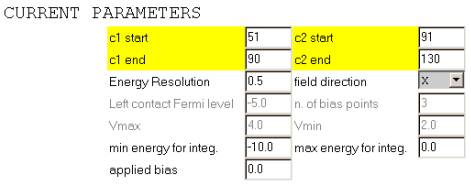c1 start / c1 end = number of the first / last atom of contact 1 c2 start / c2 end = number of the first / last atom of contact 2 Energy Resolution = energy resolution for conductance plot in eV field direction = field direction of the related applied bias min energy for integ. = min energy for conductance plot in eV max energy for integ. = max energy for conductance plot in eV applied bias = applied bias in Volt

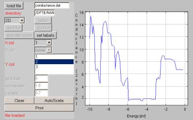
After setting these parameters you can save the profile and/or submit the calculation by pressing do computation. The output file of the calculation will be the conductance.dat file which contains the conductance of the structure. Additionally the program calculates the surface density of the states of the two contacts (surface.dat) files.

Current

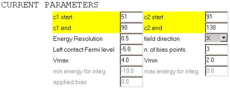
If you are interested to Current calculations click on the current button. New fields will be activated

c1 start / c1 end = number of the first / last atom of contact 1 c2 start / c2 end = number of the first / last atom of contact 2 Energy Resolution = energy resolution for integration in eV Field direction = field direction of the related applied bias Left contact Fermi Level. = Fermi Level of the left (1) contact in eV n. of bias points = number of bias points Vmax / Vmin = value of max / min applied bias in Volt

After setting these parameters you can save the profile and/or submit the calculation by pressing do computation. The output file of the calculation will be the IV.dat file which contains the current characteristics of the structure. Moreover you will have the tunneling_###.dat files which contains the tunneling coefficient for each ### bias point. Additionally the program calculates the surface density of the states of the two contacts (surface_###.dat) files.

Step 7: Monitoring the job execution

After the job has been submitted you can monitor the job execution by clicking on the Jobs Status link in the left frame, just above the list of the Services (simulators). For details on this see the relative documentation: Job Monitor Utility.

Step 8: Plot

Results of the simulation can be either plotted using the ICODE Hyperplot tool or downloaded on the CLIENT computer.